12.2 Simulated Annealing
Annealing is the process of heating a metal or glass to remove imperfections and improve strength in the material. When metal is hot, the particles are rapidly rearranging at random within the material. The random rearrangement helps to strengthen weak molecular connections. As the material cools, the random particle rearrangement continues, but at a slower rate. The overall process is governed by time and the material’s energy at a particular time.
The annealing process that happens to particles within a material can be abstracted and applied for the purpose of feature selection. The goal in this case is to find the strongest (or most predictive) set of features for predicting the response. In the context of feature selection, a predictor is a particle, the collection of predictors is the material, and the set of selected features in the current arrangement of particles. To complete the analogy, time is represented by iteration number, and the change in the material’s energy is the change in the predictive performance between the current and previous iteration. This process is called simulated annealing (Kirkpatrick, Gelatt, and Vecchi 1983; Van Laarhoven and Aarts 1987).
To initialize the simulated annealing process, a subset of features are selected at random. The number of iterations is also chosen. A model is then built and the predictive performance is calculated. Then a small percentage (1-5) of features are randomly included or excluded from the current feature set and predictive performance is calculated for the new set. If performance improves with the new feature set, then the new set of features is kept. However, if the new feature set has worse performance, then an acceptance probability is calculated using the formula
\[Pr[accept] = \exp\left[-\frac{i}{c}\left(\frac{old-new}{old}\right)\right]\]
in the case where better performance is associated with larger values. The probability is a function of time and change in performance, as well as a constant, \(c\) which can be used to control the rate of feature perturbation. By default, \(c\) is set to 1. After calculating the acceptance probability, a random uniform number is generated. If the random number is greater than the acceptance probability, then the new feature set is rejected and the previous feature set is used. Otherwise, the new feature set is kept. The randomness imparted by this process allows simulated annealing to escape local optimums in it search for the global optimum.
To understand the acceptance probability formula, consider an example where the objective is to optimize predictive accuracy. Suppose the previous solution had an accuracy of 85% and the current solution had an accuracy of 80%. The proportionate decrease of the current solution relative to the previous solution is 0.059. If this situation occurred in the first iteration, then the acceptance probability would be 0.94. If this situation occurred at iteration 5, the probability of accepting the inferior subset would be 0.75%. At iteration 50, this the acceptance probability drops to 0.05. Therefore, the probability of accepting a worse solution decreases as the algorithm iteration increases.
This algorithm summarizes the basic simulated annealing algorithm for feature selection:
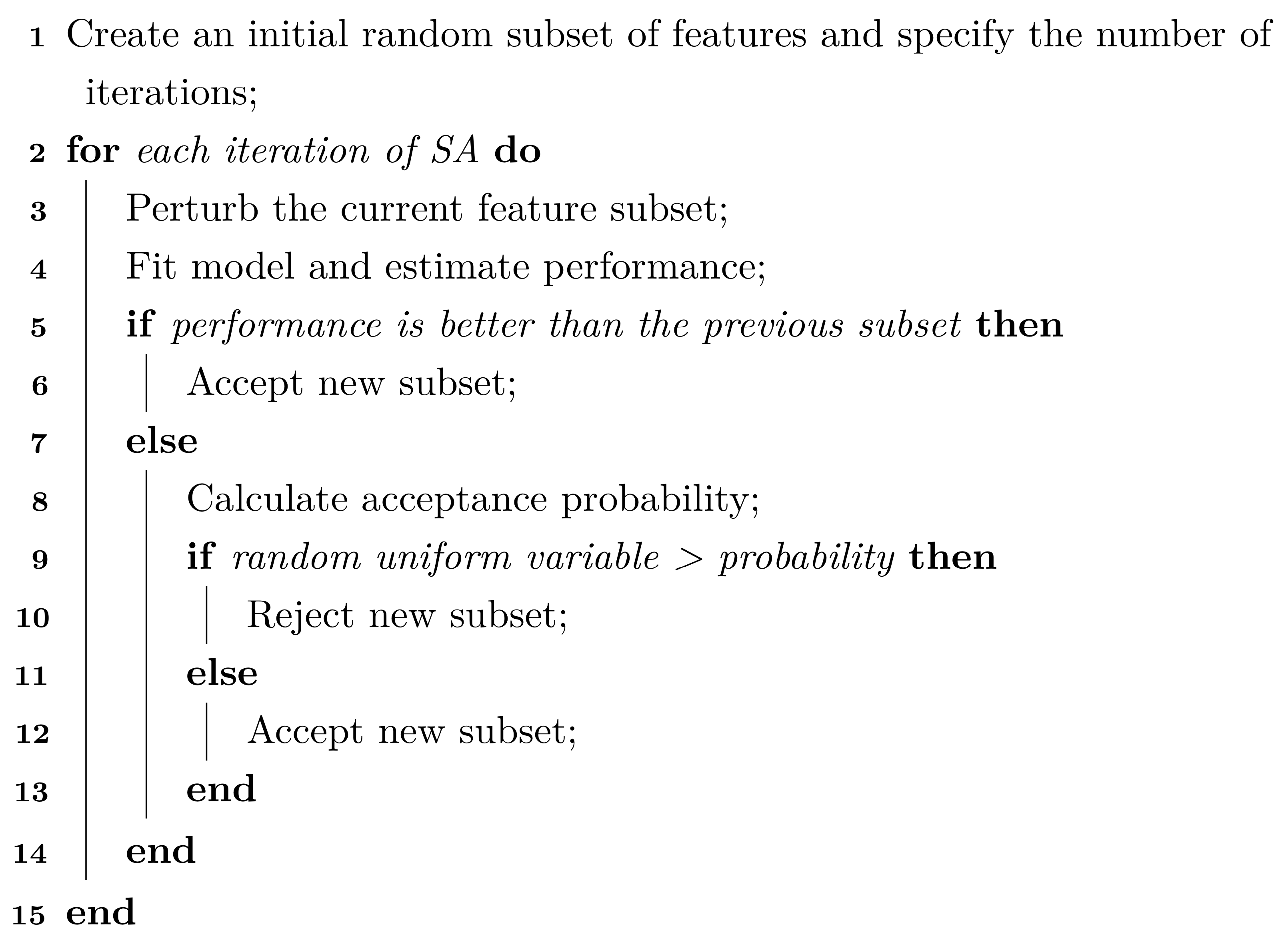
While the random nature of the search and the acceptance probability criteria help the algorithm avoid local optimums, a modification called restarts provides and additional layer of protection from lingering in inauspicious locales. If a new optimal solution has not been found within \(I\) iterations, then the search resets to the last known optimal solution and proceeds again with \(i\) being the number of iterations since the restart.
As an example, the table below shows the first 15 iterations of simulated annealing where the outcome is the area under the ROC curve. The restart threshold was set to 10 iterations. The first two iterations correspond to improvements. At iteration three, the area under the ROC curve does not improve but the loss is small enough to have a corresponding acceptance probability of 95.8%. The associated random number is smaller, so the solutions is accepted. This pays off since the next iteration results in a large performance boost but is followed by a series of losses. Note that, at iteration six, the loss is large enough to have an acceptance probability of 82.6% which is rejected based on the associated draw of a random uniform. This means that configuration seven is based on configuration number five. These losses continue until iteration 14 where the restart occurs; configuration 15 is based on the last best solution (at iteration four).
| Iteration | Size | ROC | Probability | Random Uniform | Status |
|---|---|---|---|---|---|
| 1 | 122 | 0.776 | — | — | Improved |
| 2 | 120 | 0.781 | — | — | Improved |
| 3 | 122 | 0.770 | 0.958 | 0.767 | Accepted |
| 4 | 120 | 0.804 | — | — | Improved |
| 5 | 120 | 0.793 | 0.931 | 0.291 | Accepted |
| 6 | 118 | 0.779 | 0.826 | 0.879 | Discarded |
| 7 | 122 | 0.779 | 0.799 | 0.659 | Accepted |
| 8 | 124 | 0.776 | 0.756 | 0.475 | Accepted |
| 9 | 124 | 0.798 | 0.929 | 0.879 | Accepted |
| 10 | 124 | 0.774 | 0.685 | 0.846 | Discarded |
| 11 | 126 | 0.788 | 0.800 | 0.512 | Accepted |
| 12 | 124 | 0.783 | 0.732 | 0.191 | Accepted |
| 13 | 124 | 0.790 | 0.787 | 0.060 | Accepted |
| 14 | 124 | 0.778 | — | — | Restart |
| 15 | 120 | 0.790 | 0.982 | 0.049 | Accepted |
12.2.1 Selecting Features without Overfitting
How should the data be used for this search method? Based on the discussion in Section 10.4, it was noted that the same data should not be used for selection, modeling, and evaluation. An external resampling procedure should be used to determine how many iterations of the search are appropriate. This would average the assessment set predictions across all resamples to determine how long the search should proceed when it is directly applied to the entire training set. Basically, the number of iterations is a tuning parameter.
For example, if 10-fold cross-validation is used as the external resampling scheme, simulated annealing is conducted 10 times on 90% of the data. Each corresponding assessment set is used to estimate how well the process is working at each iteration of selection.
Within each external resample, the analysis set is available for model fitting and assessment. However, it is probably not a good idea to use it for both purposes. A nested resampling procedure would be more appropriate An internal resample of the data should be used to split it into a subset used for model fitting and another for evaluation. Again, this can be a full iterative resampling scheme or a simple validation set. Again suppose 10-fold cross-validation is used for the external resample. If the external analysis set, which is 90% of the training set, is larger enough we might use a random 80% of these data for modeling and 20% for evaluation. These would be the internal analysis and assessment sets, respectively. The latter is used to guide the selection process towards an optimal subset. A diagram of the external and internal cross-validation approach is illustrated in Figure 12.2.

Figure 12.2: A diagram of external and internal cross-validation for global search.
Once the external resampling is finished, there are matching estimates of performance for each iteration of simulated annealing and each serves a different purpose:
the internal resamples guide the subset selection process
the external resamples help tune the number of search iterations to use.
For data sets with many training set samples, the internal and external performance measures may track together. In smaller data sets, it is not uncommon for the internal performance estimates to continue to show improvements while the external estimates are flat or become worse. While the use of two levels of data splitting is less straightforward and more computationally expensive, it is the only way to understand if the selection process is overfitting.
Once the optimal number of search iterations is determined, the final simulated annealing search is conducted on the entire training set. As before, the same data set should not be used to create the model and estimate the performance. An internal split is still required.
From this last search, the optimal predictor set is determined and the final model is fit to the entire training set using the optimal predictor set.
This resampled selection procedure is summarized in this algorithm:
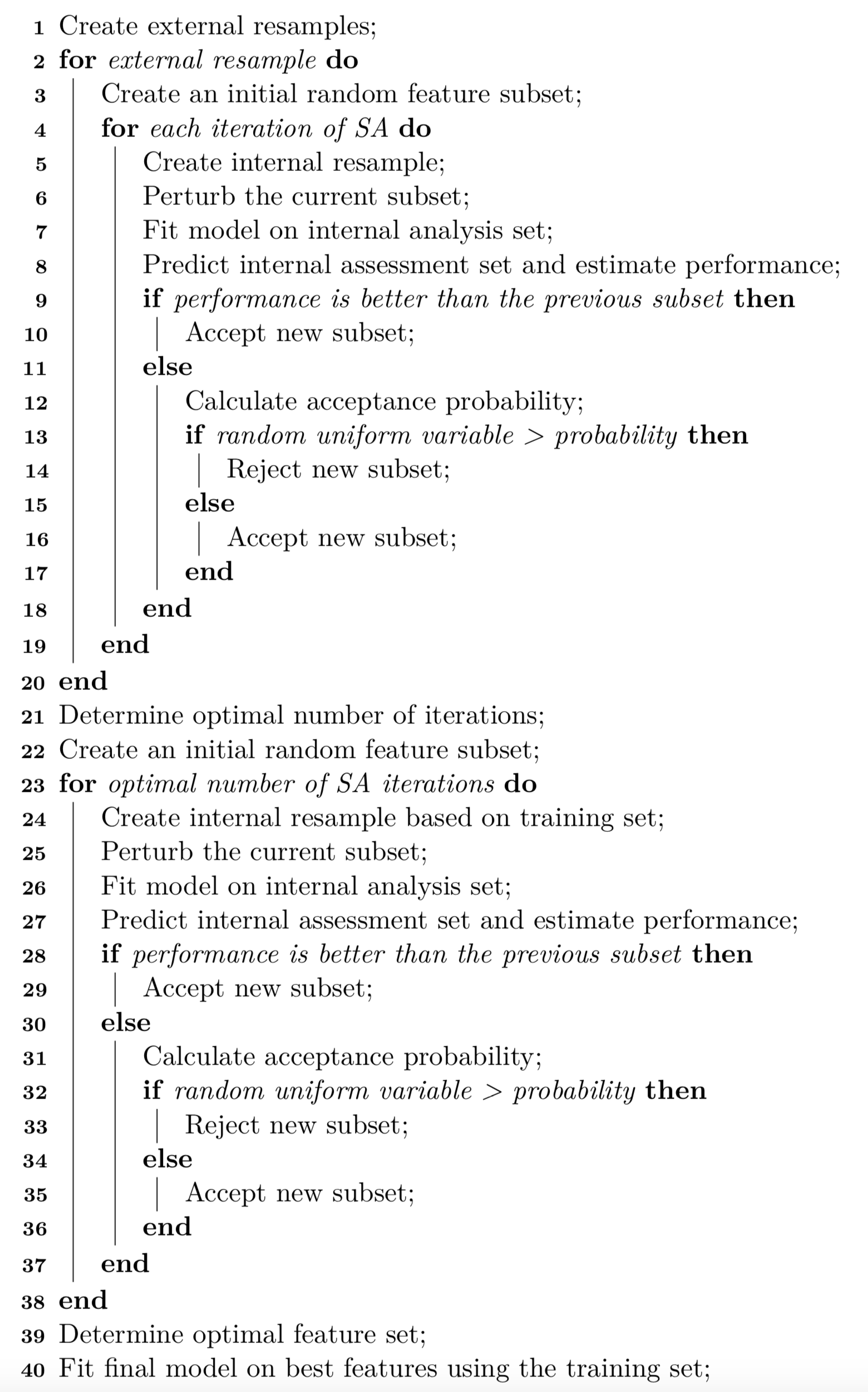
It should be noted that lines 2–20 can be run in parallel (across external resamples) to reduce the computational time required.
12.2.2 Application to Modeling the OkCupid Data
To illustrate this process, the OkCupid data are used. Recall that the training set includes 38,809 profiles, including 7,167 profiles that are reportedly in the STEM fields. As before, we will use 10-fold cross-validation as our external resampling procedure. This results in 6,451 STEM profiles and 28,478 other profiles being available for modeling and evaluation. If a validation set of 10% of these data were applied, there would be 646 STEM profiles and 2,848 other profiles on hand to estimate the area under the ROC curve and other metrics. Since there are fewer STEM profiles, sensitivity computed on these data would reflect the highest amount of uncertainty. Supposing that a model could achieve 80% sensitivity, the width of the 90% confidence interval for this metric would be 6.3\(\%\). Although subjective, this seems precise enough to be used to guide the simulated annealing search reliably.
A naive Bayes model will be used to illustrate the potential utility of this search method. 500 iterations of simulated annealing will be used with restarts occurring after 10 consecutive suboptimal feature sets have been found. The area under the ROC curve is used to optimize the models and to find the optimal number of SA iterations. To start, we initialize the first subset by randomly selecting half of the possible predictors (although this will be investigated in more detail below).
Let’s first look at how the searches did inside the external resampling loop. Figure 12.3 shows how the internal ROC estimates changed across the 10 external resamples. The trends vary; some show an increasing trend in performance across iterations while others appear to change very little across iterations. This reflects that there can be substantial variation in the selection process even for data sets with almost 35,000 data points being used within each resample. The last panel shows these values averaged across all resamples.

Figure 12.3: Internal performance profile for naive Bayes models selected via simulated annealing for each external resample.
The external resamples also have performance estimates for each iteration. Are these consistent with the inner validations sets? The average rank correlation between the two sets of ROC statistics is 0.622 with a range of (0.43, 0.85). This indicates fairly good consistency. Figure 12.4 overlays the separate internal and external performance metrics averaged across iterations of the search. The cyclical patterns seen in these data reflect the restart feature of the algorithm. The best performance was associated with 383 iterations but it is clear that other choices could be made without damaging performance. Looking at the individual resamples, the optimal iterations ranged from 69 to 404 with an average of 258 iterations. While there is substantial variability in these values, the number of variables selected at those points in the process are more precise; the average was 56 predictors with a range of (49, 64). As will be shown below in Figure 12.7, the size trends across iterations varied with some resamples increasing the number of predictors while others decreased.

Figure 12.4: Performance profile for naive Bayes models selected via simulated annealing where a random 50 percent of the features were seeded into the initial subset.
Now that we have a sense of how many iterations of the search are appropriate, let’s look at the final search. For this application of SA, we mimic what was done inside of the external resamples; a validation set of 10% is allocated from the training set and the remainder is used for modeling. Figure 12.5 shows the trends for both the ROC statistic as well as the subset size over the maximum 383 iterations. As the number of iterations increases, subset size trends downwards and the area under the ROC curve trends slowly upwards. During this final search, the iteration with the best area under the ROC curve (0.837) was 356 where 63 predictors were used.

Figure 12.5: Trends for the final SA search using the entire training set and a 10 percent internal validation set.
In the end, 66 predictors (out of a possible 110) were selected and used in the final model:
| diet | education | height | income | time since last on-line |
| offspring | pets | religion | smokes | town |
| ‘speaks’ C++ fluently | cpp_okay | ‘speaks’ C++ poorly | lisp | ‘speaks’ lisp poorly |
| black | hispanic/latin | indian | middle_eastern | native_american |
| other | pacific_islander | essay_length |
software
|
engineer
|
startup
|
tech
|
computers
|
engineering
|
computer
|
internet
|
science
|
technical
|
web
|
programmer
|
scientist
|
code
|
lol
|
biotech
|
matrix
|
geeky
|
solving
|
teacher
|
student
|
silicon
|
law
|
electronic
|
mobile
|
systems
|
electronics
|
futurama
|
alot
|
firefly
|
valley
|
lawyer
|
| the number of exclaims | the number of extraspaces | the number of lowersp | the number of periods | the number of words |
| sentiment score | the number of first person text | the percentage of first person | the number of second-person (possessive) text | the number of ‘to be’ occurances |
| the number of prepositions |
Based on external resampling, our estimate of performance for this model was an ROC AUC of 0.799. This is slightly better than the full model that was estimated in Section 12.1. The main benefit to this process was to reduce the number of predictors. While performance was maintained in this case, performance may be improved in other cases.
A randomization approach was used to investigate if the 52 selected features contained good predictive information. For these data, 100 random subsets of size 66 were generated and used as input to naive Bayes models. The performance of the model from SA was better than 95% of the random subsets. This result indicates that SA selection process approach can be used to find good predictive subsets.
12.2.3 Examining Changes in Performance
Simulated annealing is a controlled random search; the new candidate feature subset is selected completely at random based on the current state. After a sufficient number of iterations, a data set can be created to quantify the difference in performance with and without each predictor. For example, for a SA search lasting 500 iterations, there should be roughly 250 subsets with and without each predictor and each of these has an associated area under the ROC curve computed from the external holdout set. A variety of different analyses can be conducted on these values but the simplest is a basic t-test for equality. Using the SA that was initialized with half of the variables, the 10 predictors with the largest absolute t statistics were (in order): education level, software, engineer keyword, income, the number of words, startup, solving, the number of characters/word, height, and the number of lower space characters. Clearly, a number of these predictors are related and measure characteristics connected to essay length. As an additional benefit to identifying the subset of predictive features, this post hoc analysis can be used to get a clear sense of the importance of the predictors.
12.2.4 Grouped Qualitative Predictors Versus Indicator Variables
Would the results be different if the categorical variables were converted to dummy variables? The same analysis was conducted where the initial models were seeded with half of the predictor set. As with the similar analyses conducted in Section 5.7, all other factors were kept equal. However, since the the number of predictors increased from 110 to 298, the number of search iterations was increase from 500 to 1,000 to make sure that all predictors had enough exposure to the selection algorithm. The results are shown in Figure 12.6. The extra iterations were clearly needed to help to achieve a steady state of predictive performance. However, the model performance was slightly worse (AUC: 0.801) than the approach that kept the categories in a single predictor (AUC: 0.799).

Figure 12.6: Results when qualitative variables are decomposed into individual predictors.
12.2.5 The Effect of the Initial Subset
On additional aspect that is worth considering: how did the subset sizes change within external resamples and would these trends be different if the initial subset had been seeded with more (or less) predictors? To answer this, the search was replicated with initial subsets that were either 10% or 90% of the total feature set. Figure 12.7 shows the smoothed subset sizes for each external resample colored by the different initial percentages. In many instances, the three configurations converged to a subset size that was about half of the total number of possible predictors (although a few showed minimal change overall). A few of the large initial subsets resulted in larger subsets in the end while the smaller initial models tended to drive upward to the middle. There is some consistency across the three configurations but it does raise the potential issue of how forcefully simulated annealing will try to reduce the number of predictors in the model.

Figure 12.7: Resampling trends across iterations for different initial feature subset sizes. These results were achieved using simulated annealing applied to the OkCupid data.
In terms of performance, the areas under the ROC curves for the three sets were 0.805 (10%), 0.799 (50%), and 0.804 (90%). Given the variation in these results, there was no appreciable difference in performance across the different settings.