4.1 Introduction to the Chicago Train Ridership Data
To illustrate how exploratory visualizations are a critical part of understanding a data set and how visualizations can be used to identify and uncover representations of the predictors that aid in improving the predictive ability of a model, we will be using data collected on ridership on the Chicago Transit Authority (CTA) “L” train system36 (Figure 4.1). In the short term, understanding ridership over the next one or two weeks would allow the CTA to ensure that an optimal number of cars were available to service the Chicagoland population. As a simple example of demand fluctuation, we would expect that ridership in a metropolitan area would be stronger on weekdays and weaker on weekends. Two common mistakes of misunderstanding demand could be made. At one extreme, having too few cars on a line to meet weekday demand would delay riders from reaching their destination and would lead to overcrowding and tension. At the other extreme, having too many cars on the weekend would be inefficient leading to higher operational costs and lower profitability. Good forecasts of demand would help the CTA to get closer to optimally meeting demand.
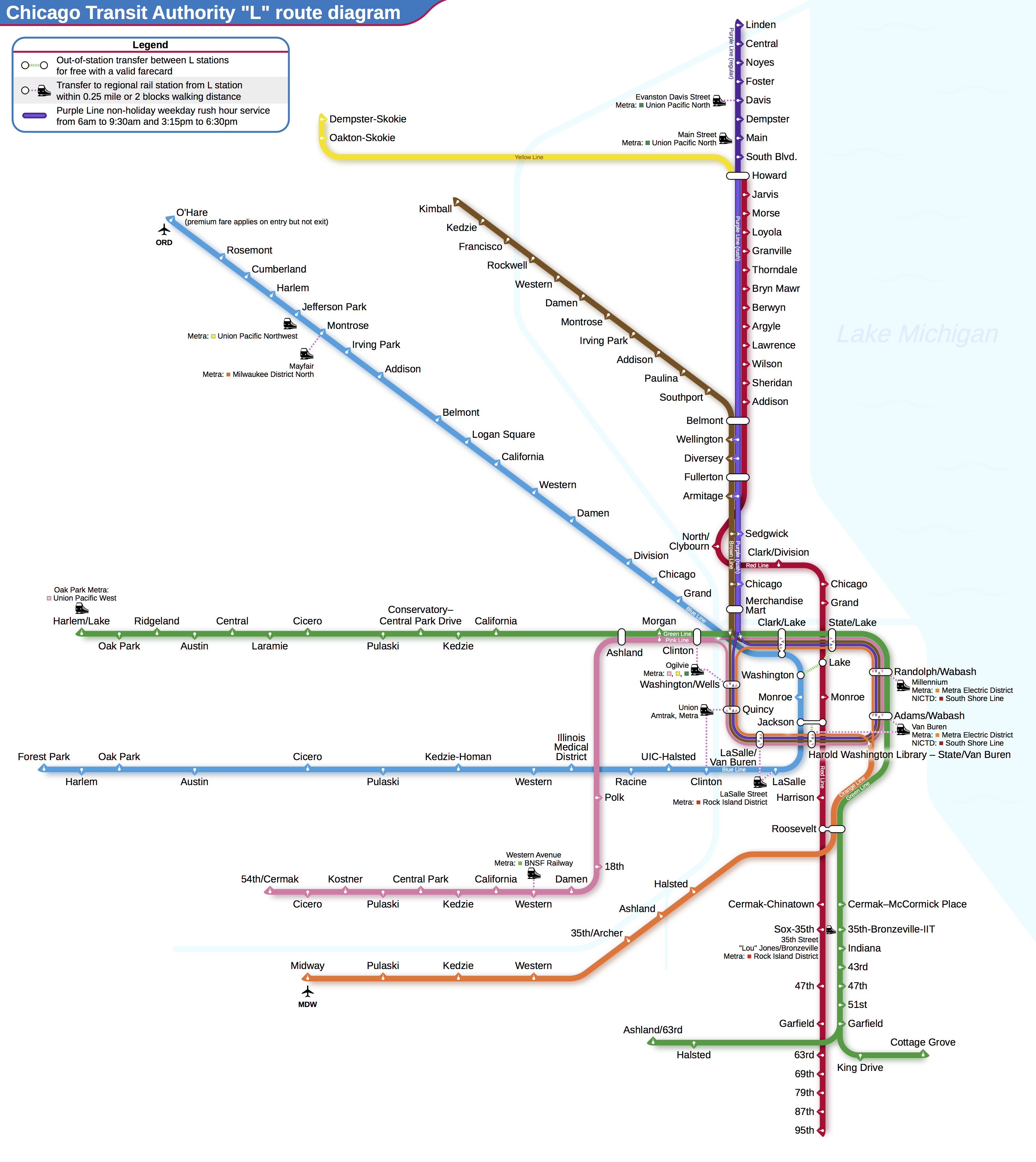
Figure 4.1: Chicago Transit Authority ‘L’ map. For this illustration, we are interesting in predicting the ridership at the Clark/Lake station in the Chicago Loop. (Source: Wikimedia Commons, Creative Commons license)
In the long term, forecasting could be used to project when line service may be necessary, to change the frequency of stops to optimally service ridership, or to add or eliminate stops as populations shift and demand strengthens or weakens.
For illustrating the importance of exploratory visualizations, we will focus on short-term forecasting of daily ridership. Daily ridership data were obtained for 126 stations37 between January 22, 2001 and September 11, 2016. Ridership is measured by the number of entries into a station across all turnstiles, and the number of daily riders across stations during this time period varied considerably, ranging between 0 and 36,323 per day. For ease of presentation, ridership will be shown and analyzed in units of thousands of riders.
Our illustration will narrow to predicting daily ridership at the Clark/Lake stop. This station is an important stop to understand; it is located in the downtown loop, has one of the highest riderships across the train system, and services four different lines covering northern, western, and southern Chicago.
For these data, the ridership numbers for the other stations might be important to the models. However, since the goal is to predict future ridership volume, only historical data would be available at the time of prediction. For time series data, predictors are often formed by lagging the data. For this application, when predicting day \(D\), predictors were created using the lag–14 data from every station (e.g., ridership at day \(D-14\)). Other lags can also be added to the model, if necessary.
Other potential regional factors that may affect public transportation ridership are the weather, gasoline prices, and the employment rate. For example, it would be reasonable to expect that more people would use public transportation as the cost of using personal transportation (i.e., gas prices) increase for extended periods of time. Likewise, the use of public transportation would likely increase as the unemployment rate decreases. Weather data were obtained for the same time period as the ridership data. The weather information was recorded hourly and included many conditions such as overcast, freezing rain, snow, etc.. A set of predictors were created that reflects conditions related to rain, snow/ice, clouds, storms, and clear skies. Each of these categories is determined by pooling more granular recorded conditions. For example, the rain predictor reflects recorded conditions that included “rain,” “drizzle,” and “mist”. New predictors were encoded by summarizing the hourly data across a day by calculating the percentage of observations within a day where the conditions were observed. As an illustration, on December 20, 2012, conditions were recorded as snowy (12.8% of the day), cloudy (15.4%), as well as stormy (12.8%), and rainy (71.8%). Clearly, there is some overlap in the conditions that make up these categories, such as cloudy and stormy.
Other hourly weather data were also available related to the temperature, dew point, humidity, air pressure, precipitation and wind speeds. Temperature was summarized by the daily minimum, median, and maximum as well as the daily change. Pressure change was similarly calculated. In most other cases, the median daily value was used to summarize the hourly records. As with the ridership data, future weather data are not available so lagged versions of these data were used in the models38. In total, there were 18 weather-related predictors available. Summarization of these types of data are discussed more in Chapter 9.
In addition to daily weather data, average weekly gasoline prices were obtained for the Chicago region (U.S. Energy Information Administration 2017a) from 2001 through 2016. For the same time period, monthly unemployment rates were pulled from United States Census Bureau (2017). The potential usefulness of these predictors will be discussed below.