9 Working with Profile Data
Let’s review the previous data sets in terms of what has been predicted:
the price of a house in Iowa
daily train ridership at Clark and Lake
the species of a feces sample collected on a trail
a patient’s probability of having a stroke
From these examples, the unit of prediction is fairly easy to determine because the data structures are simple. For the housing data, we know the location, structural characteristics, last sale price, and so on. The data structure is straightforward: rows are houses and columns are fields describing them. There is one house per row and, for the most part, we can assume that these houses are statistically independent of one another. In statistical terms, it would be said that the houses are the independent experimental unit of data. Since we make predictions on the properties (as opposed to the ZIP code or other levels of aggregation), the properties are the unit of prediction.
This may not always be the case. As a slight departure, consider the Chicago train data. The data set has rows corresponding to specific dates and columns are characteristics of these days: holiday indicators, ridership at other stations a week prior, and so on. Predictions are made daily; this is the unit of prediction. However, recall they there are also weather measurements. The weather data was obtained multiple times per day, usually hourly. For example, on January 5, 2001 the first 15 measurements are
| Time | Temp | Humidity | Wind | Conditions |
|---|---|---|---|---|
| 00:53 | 27.0 | 92 | 21.9 | Overcast |
| 01:53 | 28.0 | 85 | 20.7 | Overcast |
| 02:53 | 27.0 | 85 | 18.4 | Overcast |
| 03:53 | 28.0 | 85 | 15.0 | Mostly Cloudy |
| 04:53 | 28.9 | 82 | 13.8 | Overcast |
| 05:53 | 32.0 | 79 | 15.0 | Overcast |
| 06:53 | 33.1 | 78 | 17.3 | Overcast |
| 07:53 | 34.0 | 79 | 15.0 | Overcast |
| 08:53 | 34.0 | 61 | 13.8 | Scattered Clouds |
| 09:53 | 33.1 | 82 | 16.1 | Clear |
| 10:53 | 34.0 | 75 | 12.7 | Clear |
| 11:53 | 33.1 | 78 | 11.5 | Clear |
| 12:53 | 33.1 | 78 | 11.5 | Clear |
| 13:53 | 32.0 | 79 | 11.5 | Clear |
| 14:53 | 32.0 | 79 | 12.7 | Clear |
These hourly data are not on the unit of prediction (daily). We would expect that, within a day, the hourly measurements are more correlated with each other than they would be with any other random weather measurements taken at random from the entire data set. For this reason, these measurements are statistically dependent76.
Since the goal is to make daily predictions, the profile of within-day weather measurements should be somehow summarized at the day level in a manner that preserves the potential predictive information. For this example, daily features could include the mean or median of the numeric data and perhaps the range of values within a day. For the qualitative conditions, the percentage of the day that was listed as “Clear”, “Overcast”, etc. can be calculated so that weather conditions for a specific day are incorporated into the data set used for analysis.
As another example, suppose that the stroke data were collected when a patient was hospitalized. If the study contained longitudinal measurements over time we might be interested in predicting the probability of a stroke over time. In this case, the unit of prediction is the patient on a given day but the independent experimental unit is just the patient.
In some case, there can be multiple hierarchical structures. For online education, there would be interest in predicting what courses a particular student could complete successfully. For example, suppose there were 10,000 students that took the online “Data Science 101” class (labeled DS101). Some were successful and other were not. These data can be used to create an appropriate model at the student level. To engineer features for the model, the data structures should be considered. For students, possible predictors might be demographic (e.g., age, etc.) while others would be related to their previous experiences with other classes. If they had successfully completed 10 other courses, it is reasonable to think that they would more more likely to do well than if they did not finish 10 courses. For students who took DS101, a more detailed data set might look like:
| Student | Course | Section | Assignment | Start_Time | Stop_Time |
|---|---|---|---|---|---|
| Marci | STAT203 | 1 | A | 07:36 | 08:13 |
| : | : | : | B | 13:38 | 18:01 |
| : | : | : | : | : | : |
| Marci | CS501 | 4 | Z | 10:40 | 10:59 |
| David | STAT203 | 1 | A | 18:26 | 19:05 |
| : | : | : | : | : | : |
The hierarchical structure is assignment-within-section-within-course-within-student. If both STAT203 and CS501 are prerequisites for DS101, it would be safe to assume that a relatively complete data set could exist. If that is the case, then very specific features could be created such as “is the time to complete the assignment on computing a t-test in STAT203 predictive of their ability to pass or complete the data science course?”. Some features could be rolled-up at the course level (e.g., total time to complete course CS501) or at the section level. The richness of this hierarchical structure enables some interesting features in the model but it does pose the question “are there good and bad ways of summarizing profile data?”.
Unfortunately, the answer to this question depends on the nature of the problem and the profile data. However, there are some aspects that can be considered regarding the nature of variation and correlation in the data.
High content screening (HCS) data in biological sciences is another example (Giuliano et al. 1997; Bickle 2010; Zanella, Lorens, and Link 2010). To obtain this data, scientists treat cells using a drug and then measure various characteristics of the cells. Examples are the overall shape of the cell, the size of the nucleus, and the amount of a particular protein that is outside the nucleus.
HSC experiments are usually carried out on microtiter plates. For example, the smallest plate has 96 wells that can contain different liquid samples (usually in a 8 by 12 arrangement, such as in Figure 9.1). A sample of cells would be added to each well along with some treatment (such as a drug candidate). After treatment, the cells are imaged using a microscope and a set of images are taken within each well, usually at specific locations (Holmes and Huber 2019). Let’s say that, one average, there are 200 cells in an image and 5 images are taken per well. It is usually safe to pool the images within a cell so that the data structure is then cell within well within plate. Each cell is quantified using image analysis so that the underlying features are at the cellular level.
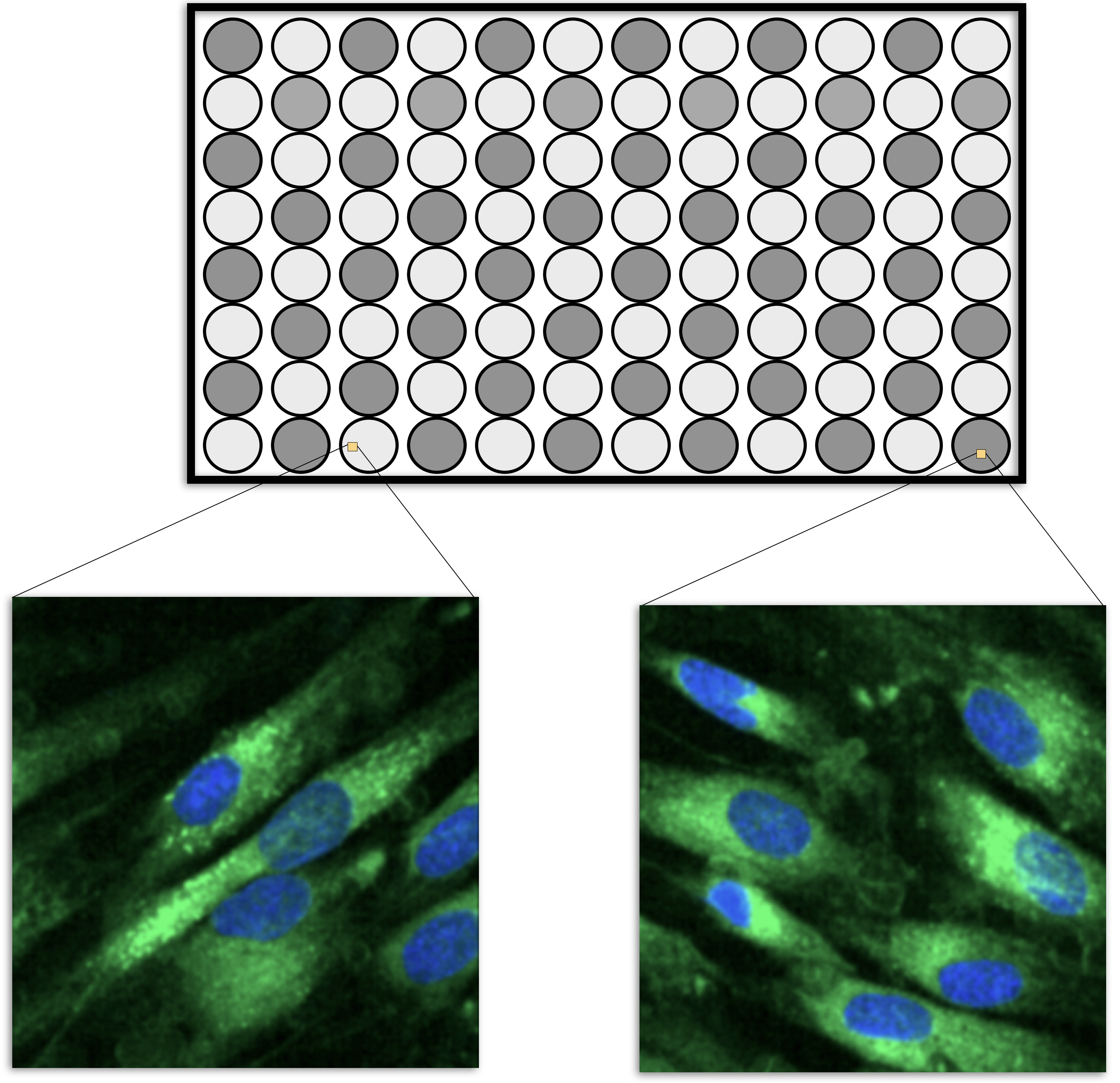
Figure 9.1: A schematic for the micro-titer plates in high content screening. The dark wells might be treated cells while the lightly colored cell would be controls. Multiple images are taken within each well and the cells in each image are isolated and quantified in different ways. The green represents the cell boundary and the blue describes the nucleus.
However, to make predictions on a drug, the data needs to be summarized to the wellular level (i.e., within the well). One method to do this would be to take simple averages and standard deviations of the cell properties, such as the average nucleus size, the average protein abundance, etc. The problem with this approach is that it would break the correlation structure of the cellular data. It is common for cell-level features to be highly correlated. As an obvious example, the abundance of a protein in a cell is correlated with the total size of the cell. Suppose that cellular features \(X\) and \(Y\) are correlated. If an important feature of these two values is their difference, then there are two ways of performing the calculation. The means, \(\bar{X}\) and \(\bar{Y}\), could be computed within the well, then the difference between the averages could be computed. Alternatively, the differences could be computed for each cell (\(D_i = X_i- Y_i\)) and then these could be averaged (i.e., \(\bar{D}\)). Does it matter? If \(X\) and \(Y\) are highly correlated, it makes a big difference. From probability theory, we know that the variance of a difference is:
\[Var[X-Y] = Var[X] + Var[Y] - 2 Cov[X, Y]\]
If the two cellular features are correlated, the covariance can be large. This can result in a massive reduction of variance if the features are differenced and then averaged at the wellular level. As noted by Wickham and Grolemund (2016):
“If you think of variation as a phenomenon that creates uncertainty, covariation is a phenomenon that reduces it.”
Taking the averages and then differences ignores the covariance term and results in noisier features.
Complex data structures are very prevalent in medical studies. Modern measurement devices such as actigraphy monitors and magnetic resonance imaging (MRI) scanners can generate hundreds of measurements per subject in a very short amount of time. Similarly, medical devices such as an electroencephalogram (EEG) or electrocardiogram (ECG) can provide a dense, continuous stream of measurements related to a patient’s brain or heart activity. These measuring devices are being increasingly incorporated into medical studies in an attempt to identify important signals that are related to the outcome. For example, Sathyanarayana et al. (2016) used actigraphy data to predict sleep quality, and Chato and Latifi (2017) examined the relationship between MRI images and survival in brain cancer patients.
While medical studies are more frequently utilizing devices that can acquire dense, continuous measurements, many other fields of study are collecting similar types of data. In the field of equipment maintenance, Caterpillar Inc. collects continuous, real-time data on deployed machines to recommend changes that better optimize performance (Marr 2017).
To summarize, some complex data sets can have multiple levels of data hierarchies which might need to be collapsed so that the modeling data set is consistent with the unit of prediction. There are good and bad ways of summarizing the data, but the tactics are usually subject-specific.
The remainder of this chapter is an extended case study where the unit of prediction has multiple layers of data. It is a scientific data set where there are a large number of highly correlated predictors, a separate time effect, and other factors. This example, like Figure 1.7, demonstrates that good preprocessing and feature engineering can have a larger impact on the results than the type of model being used.
However, to be fair, the day-to-day measurements have some degree of correlation with one another too.↩