5.4 Supervised Encoding Methods
There are several methods of encoding categorical predictors to numeric columns using the outcome data as a guide (so that they are supervised methods). These techniques are well suited to cases where the predictor has many possible values or when new levels appear after model training.
The first method is a simple translation that is sometimes called effect or likelihood encoding (Micci-Barreca 2001; Zumel and Mount 2016). In essence, the effect of the factor level on the outcome is measured and this effect is used as the numeric encoding. For example, for the Ames housing data, we might calculate the mean or median sale price of a house for each neighborhood from the training data and use this statistic to represent the factor level in the model. There are a variety of ways to estimate the effects and these will be discussed below.
For classification problems, a simple logistic regression model can be used to measure the effect between the categorical outcome and the categorical predictor. If the outcome event occurs with rate \(p\), the odds of that event is defined as \(p/(1-p)\). As an example, with the OkC data, the rate of STEM profiles in Mountain View California is 0.53 so that the odds would be 1.125. Logistic regression models the log-odds of the outcome as a function of the predictors. If a single categorical predictor is included in the model, then the log-odds can be calculated for each predictor value and can be used this as the encoding. Using the same location previously shown in Table 5.1, the simple effect encodings for the OkC data are shown in Table 5.2 under the heading of “Raw”.
| Location | Rate | n | Raw | Shrunk | Feat 1 | Feat 2 | Feat 3 |
|---|---|---|---|---|---|---|---|
| belvedere tiburon | 0.086 | 35 | -2.367 | -2.033 | 0.050 | -0.003 | 0.003 |
| berkeley | 0.163 | 2676 | -1.637 | -1.635 | 0.059 | 0.077 | 0.033 |
| martinez | 0.091 | 197 | -2.297 | -2.210 | 0.008 | 0.047 | 0.041 |
| mountain view | 0.529 | 255 | 0.118 | 0.011 | 0.029 | -0.232 | -0.353 |
| san leandro | 0.128 | 431 | -1.922 | -1.911 | -0.050 | 0.040 | 0.083 |
| san mateo | 0.277 | 880 | -0.958 | -0.974 | 0.030 | -0.195 | -0.150 |
| south san francisco | 0.178 | 258 | -1.528 | -1.554 | 0.026 | -0.014 | -0.007 |
| <new location> | -1.787 | 0.008 | 0.007 | -0.004 |
As previously mentioned, there are different methods for estimating the effects. A single generalized linear model (e.g., linear or logistic regression) can be used. While very fast, it has drawbacks. For example, what happens when a factor level has a single value? Theoretically, the log-odds should be infinite in the appropriate direction but, numerically, it is usually capped at a large (and inaccurate) value.
One way around this issue is to use some type of shrinkage method. For example, the overall log-odds can be determined and, if the quality of the data within a factor level is poor, then this level’s effect estimate can be biased towards an overall estimate that disregards the levels of the predictor. “Poor quality” could be due to a small sample size or, for numeric outcomes, a large variance within the data for that level. Shrinkage methods can also move extreme estimates towards the middle of the distribution. For example, a well-replicated factor level might have an extreme mean or log-odds (as will be seen for Mountain View data below).
A common method for shrinking parameter estimates is Bayesian analysis (McElreath 2015). In this case, expert judgement can be used prior to seeing the data to specify a prior distribution for the estimates (e.g., the means or log-odds). The prior would be a theoretical distribution that represents the overall distribution of effects. Almost any distribution can be used. If there is not a strong belief as to what this distribution should be, then it may be enough to focus on the shape of the distribution. If a bell-shaped distribution is reasonable, then a very diffuse or wide prior can be used so that it is not overly opinionated. Bayesian methods take the observed data and blend it with the prior distribution to come up with a posterior distribution that is a combination of the two. For categorical predictor values with poor data, the posterior estimate is shrunken closer to the center of the prior distribution. This can also occur when their raw estimates are relatively extreme45.
For the OkC data, a normal prior distribution was used for the log-odds that has a large standard deviation (\(\sigma = 10\)).
Table 5.2 shows the results. For most locations, the raw and shrunken estimates were very similar. For Belvedere/Tiburon, there was a relatively small sample size (and a relatively small STEM rate) and the estimate was shrunken towards the center of the prior. Note that there is a row for “<new location>”. When a new location is given to the Bayesian model, the procedure used here estimates its effect as the most likely value using the mean of the posterior distribution (a value of -1.79 for these data). A plot of the raw and shrunken effect estimates is also shown in Figure 5.2(a). Panel (b) shows the magnitude of the estimates (x-axis) versus the difference between the two. As the raw effect estimates dip lower than -2, the shrinkage pulled the values towards the center of the estimates. For example, the location with the largest log-odds value (Mountain View) was reduced from 0.118 to 0.011.
Figure 5.2: Left: Raw and shrunken estimates of the effects for the OkC data. Right: The same data shown as a function of the magnitude of the log-odds (on the x axis).
Empirical Bayes methods can also be used, in the form of linear (and generalized linear) mixed models (West and Galecki 2014). These are non-Bayesian estimation methods that also incorporate shrinkage in their estimation procedures. While they tend to be faster than the types of Bayesian models used here, they offer less flexibility than a fully Bayesian approach.
One issue with effect encoding, independent of the estimation method, is that it increases the possibility of overfitting. This is because the estimated effects are taken from one model and put into another model (as variables). If these two models are based on the same data, it is somewhat of a self-fulfilling prophecy. If these encodings are not consistent with future data, this will result in overfitting that the model cannot detect since it is not exposed to any other data that might contradict the findings. Also, the use of summary statistics as predictors can drastically underestimate the variation in the data and might give a falsely optimistic opinion of the utility of the new encoding column46. As such, it is strongly recommended that either a different data sets be used to estimate the encodings and the predictive model or that their derivation is conducted inside resampling so that the assessment set can measure the overfitting (if it exists).
Another supervised approach comes from the deep learning literature on the analysis of textual data. In this case, large amounts of text can be cut up into individual words. Rather than making each of these words into its own indicator variable, word embedding or entity embedding approaches have been developed. Similar to the dimension reduction methods described in the next chapter, the idea is to estimate a smaller set of numeric features that can be used to adequately represent the categorical predictors. Guo and Berkhahn (2016) and Chollet and Allaire (2018) describe this technique in more detail. In addition to the dimension reduction, there is the possibility that these methods can estimate semantic relationships between words so that words with similar themes (e.g., “dog”, “pet”, etc.) have similar values in the new encodings. This technique is not limited to text data and can be used to encode any type of qualitative variable.
Once the number of new features are specified, the model takes the traditional indicators variables and randomly assigns them to one of the new features. The model then tries to optimize both the allocation of the indicators to features as well as the parameter coefficients for the features themselves. The outcome in the model can be the same as the predictive model (e.g., sale price or the probability of a STEM profile). Any type of loss function can be optimized but it is common to use the root mean squared error for numeric outcomes and cross-entropy for categorical outcomes (which are the loss functions for linear and logistic regression, respectively). Once the model is fit, the values of the embedding features are saved for each observed value of the quantitative factor. These values serve as a look-up table that is used for prediction. Additionally, an extra level can be allocated to the original predictor to serve as a place-holder for any new values for the predictor that are encountered after model training.
A more typical neural network structure can be used that places one or more set of nonlinear variables positioned between the predictors and outcomes (i.e., the hidden layers). This allows the model to make more complex representations of the underlying patterns. While a complete description of neural network models is beyond the scope of this book, Chollet and Allaire (2018) provide a very accessible guide to fitting these models and specialized software exists to create the encodings.
For the OkCupid data, there are 52 locations in the training set. We can try to represent these locations, plus a slot for potential new locations, using a set embedding features. A schematic for the model is:
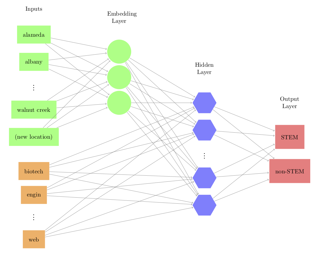
Here, each green node represents the part of the network that is dedicated to reducing the dimensionality of the location data to a smaller set. In this diagram, three embedding features are used. The model can also include a set of other predictors unrelated to the embedding components. In this diagram an additional set of indicator variables, derived later in Section 5.6, is shown in orange. This allows the embeddings to be estimated in the presence of other potentially important predictors so that they can be adjusted accordingly. Each line represents a slope coefficient for the model. The connections between the indicator variable layer on the left and the embedding layer, represented by the green circular nodes, are the values that will be used to represent the original locations. The activation function connecting the embeddings and other predictors to the hidden layer used rectified linear unit (ReLU) connections (introduced in Section 6.2.1). This allows the model additional complexity using nonlinear relationships. Here, ten hidden nodes were used during model estimation. In total, the network model estimated 678 parameters in the course of deriving the embedding features. Cross-entropy was used to fit the model and it was trained for 30 iterations, where it was found to converge. These data are not especially complex since there are few unique values that tend to have very little textual information since each data point only belongs to a single location (unlike the case where text is cut into individual words).
Table 5.2 shows the results for several locations and Figure 5.3 contains the relationship between each of the resulting encodings (i.e., features) and the raw log-odds. Each of the features has a relationship with the raw log-odds, with rank correlations of -0.01, -0.58, and -0.69. Some of the new features are correlated with the others; absolute correlation values range between 0.01 and 0.69. This raises the possibility that, for these data, fewer features might be be required. Finally, as a reminder, while an entire supervised neural network was used here, the embedding features can be used in other models for the purpose of preprocessing the location values.
Figure 5.3: Three word embedding features for each unique location in the OkC data and their relationship to the raw odds-ratios.